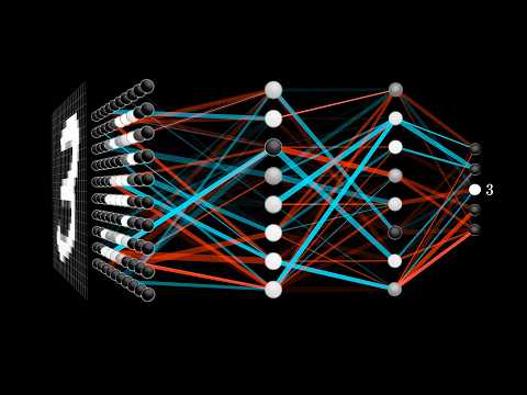
Animated math intuition by Grant Sanderson - the canonical neural network visualizations.
Cross-entropy connects information theory to compression and language modeling. Compression can reveal linguistic similarities and family trees among languages. Understanding cross-entropy enhances our approach to training language models.
The video presents a puzzle about random chords on a circle. It discusses the expected number of intersection points for 10 and 100 chords. The concept ties into Bertrand's paradox regarding random chord selection.
Claude Shannon studied how compressibility of English text relates to predictability. Shannon's experiments involved character sequences and human predictions to understand probabilities. He estimated that English could be compressed to around 1 bit per character with sufficient context. His work combined statistics, human guesswork, and the concept of entropy. The pursuit of data compression has evolved to incorporate engineered intelligence.
The video presents a puzzle involving robot movement instructions. Instructions are organized as a biased random walk with defined probabilities. Viewers are tasked with efficiently encoding these instructions in binary.
Text compression is fundamentally limited by information theory. Claude Shannon's work highlights the equivalence of prediction and compression. Compression can be viewed as a core element of intelligence.
The puzzle involves tying random ends of strings to form loops. Starting with 50 strings, the goal is to determine the average number of loops formed. The process involves randomly selecting and tying string ends together.
The puzzle involves covering 10 points on a plane with unit discs. Discs must be disjoint and cannot overlap. The challenge is to determine if all points can always be covered.
M.C. Escher's 1956 lithograph 'The Print Gallery' is a complex piece of art. It features a man looking at a picture of a boat, which leads to a paradoxical exploration of perspective. The work includes a central ambiguous hole that challenges viewers' perceptions. Mathematicians De Smit and Lenstra analyzed the image's deeper implications. Escher himself considered this piece one of his most peculiar creations.
Players must find two distinct subsets with the same sum. The game involves selecting 10 numbers from 1 to 100. The challenge is to determine if a winning strategy exists.
The video explores the connection between math and Escher's art, particularly focusing on the lithograph 'Print Gallery.' It introduces the concept of the Droste effect, which features self-similar images nested within themselves. A visual demonstration of taking a logarithm of Escher's artwork is provided to explain its unique depth and structure.
Bacteria replicate on a grid, creating a puzzle to clear lattice points. Minimum moves required scales with grid size but becomes astronomical for larger boxes. Weights of cells remain fixed and limit the ability to clear certain areas, proving some configurations impossible.
The video explores a beautiful and underappreciated mathematical formula related to dimensions and probabilities. It illustrates concepts using visualizations of geometric shapes like circles and spheres. The importance of higher dimensional geometry is discussed, highlighting its real-world applications.
The video introduces a game involving bacterial replication on a grid. The objective is to clear a specific box of all bacteria in the minimum number of moves. Replication occurs if specific conditions about adjacent spaces are met.
The ladybug clock puzzle explores probabilities in a random walk. Despite initial assumptions, all numbers from 1 to 11 are equally likely to be the last touched. The key insight involves waiting for the ladybug to touch neighboring numbers before assessing probabilities.
The Hairy Ball Theorem states it's impossible to comb hair on a ball flat without leaving at least one tuft sticking up. This theorem is illustrated through practical examples, such as programming for 3D models in video games. The formal statement involves assigning a continuous vector field to every point on the sphere, which must have at least one null vector.
A ladybug moves randomly around a clock, coloring numbers. The last number to be colored varies with different simulations. The challenge is to calculate the probability that number 6 is the last to be colored.
Laplace transforms are essential for analyzing dynamic systems influenced by external forces. They convert time-domain differential equations into algebraic forms in the s-domain. Key properties include transformation of exponential functions and linearity of the transform.
The function e^(t) is its own derivative and has significant implications for growth dynamics. Exponential functions with positive constants grow faster, while those with negative constants decay over time. When i is used as an exponent, it represents a circular motion where the velocity is always a 90° rotation of the position.
The Laplace Transform is a capable tool for solving differential equations. It breaks down functions into exponential components, aiding in understanding complex behaviors. A strong grasp of exponential functions, including complex numbers, is crucial for using Laplace Transforms.
Introduces the concept of the Laplace transform as a tool for differential equations. Explains the significance of Euler's formula and complex exponents. Visualizes exponential growth and decay through derivatives. Demonstrates the geometric interpretation of complex derivatives. Sets the stage for deeper exploration of the Laplace transform in subsequent videos.
Grant Sanderson's canonical 19-minute visual introduction to neural networks, framed around recognizing handwritten digits from MNIST. Builds up the network from scratch - input layer, two hidden layers of 16 neurons, output layer of 10 - and explains every weight, bias, and activation as you watch. Introduces the 'each layer detects edges, then patterns, then digits' hypothesis as an intuition pump, but is honest that real networks don't actually learn this neatly. Sets up the central question - how do you find the ~13,000 weights and biases - that Chapter 2 (gradient descent) answers.